SpaRV: Sparse Radiance Voxels for Scalable Geometrically Consistent LiDAR-Visual Mapping and Rendering
The University of Hong Kong
Under review
Abstract
Robotic simulation, navigation, and inspection need photorealistic and geometrically accurate maps. Radiance fields achieve photorealism, but building them from robot data raises three challenges. A robot's trajectory serves its task, not reconstruction, so images from few viewpoints leave the geometry under-constrained. Residual errors in camera poses and intrinsics blur the map. The map's GPU memory grows with scene size, which limits its level of detail in large scenes. We present SpaRV, a Sparse Radiance Voxel map rendered by differentiable ray marching, which lets irregular LiDAR scans supervise it alongside images. LiDAR depth and occupancy anchor the under-constrained geometry, and normal and smoothness regularizers keep it smooth between LiDAR points. To correct camera errors, SpaRV alternates map training with photometric optimization of the camera poses and focal lengths. To bound GPU memory in training and rendering, SpaRV holds one submap at a time at full resolution and the rest at coarser octree levels. Experiments show that SpaRV keeps the geometry consistent away from the captured trajectory and sharpens textures by optimizing the camera parameters. On one 24 GB GPU, SpaRV reconstructs a university campus captured in 63,582 images and simulates other cameras and LiDARs. We will open-source our implementation.
Video
Method
1Ray-marching rendering of sparse radiance voxels
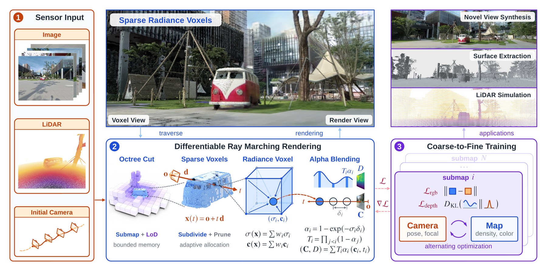
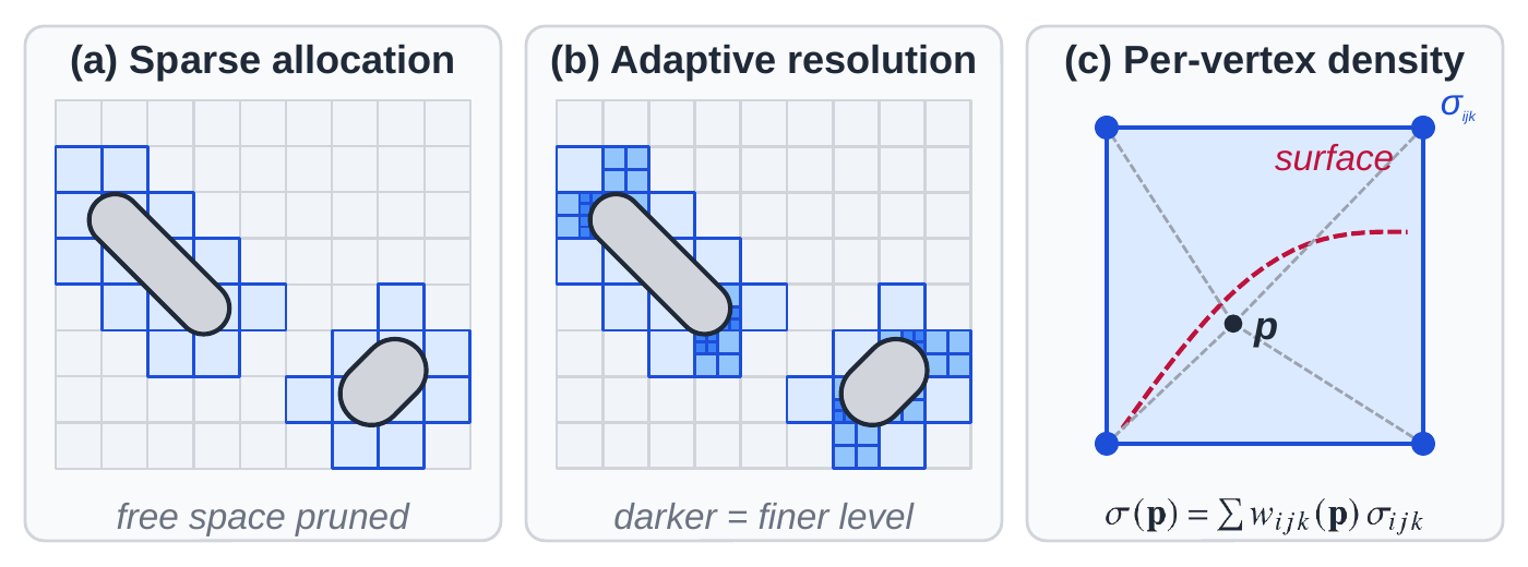
SpaRV stores the scene as sparse voxels in an octree, allocated only around surfaces and refined where more detail is needed.
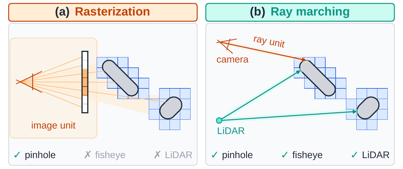
A differentiable ray marcher traverses the voxels along each ray independently. Camera pixels, LiDAR rays, and rays of non-pinhole cameras therefore supervise the map through one renderer. The rasterizer of SVRaster, in contrast, batches a pinhole pixel lattice and does not directly apply to LiDAR rays or non-pinhole cameras.
2Geometry-grounded map training
Color supervision fits every camera ray but leaves the geometry under-constrained, since different density profiles can render the same pixel color. LiDAR depth supervision anchors the field at the measured range, but only along measured rays. Between these anchors, normal and smoothness regularizers keep the surface locally smooth.
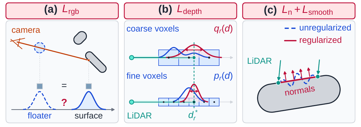
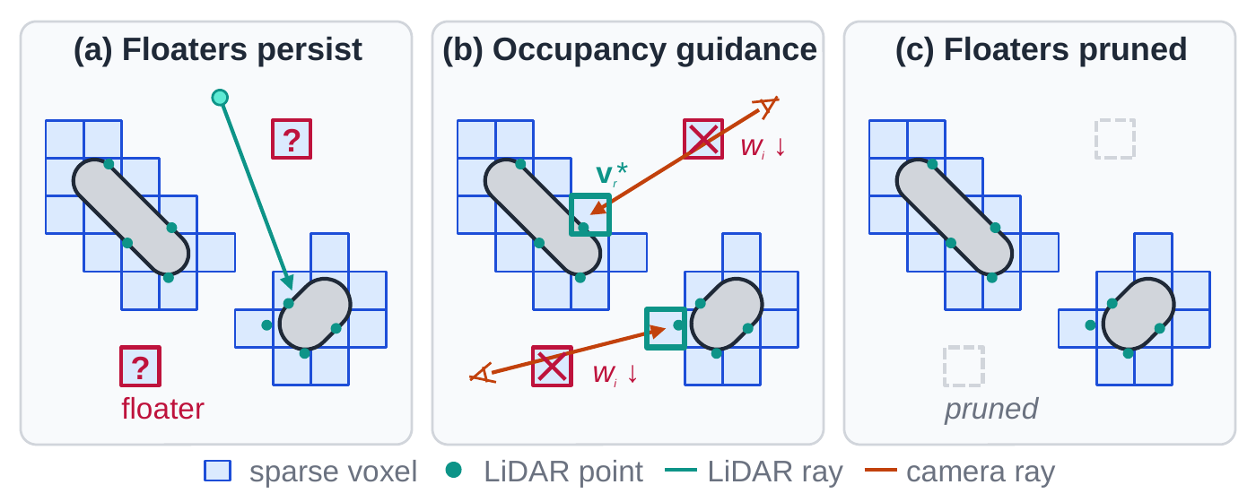
A LiDAR scan is sparse, and its field of view does not coincide with the camera's. Floaters off the measured rays therefore get no depth supervision. The point cloud still marks which voxels contain a measured surface. Occupied voxel guidance turns that occupancy into a termination target for camera rays that hit an occupied voxel.
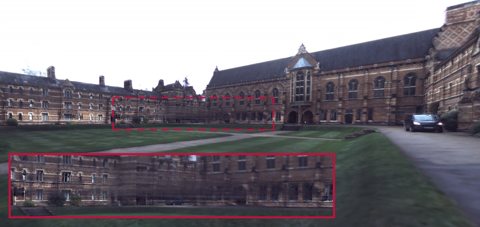
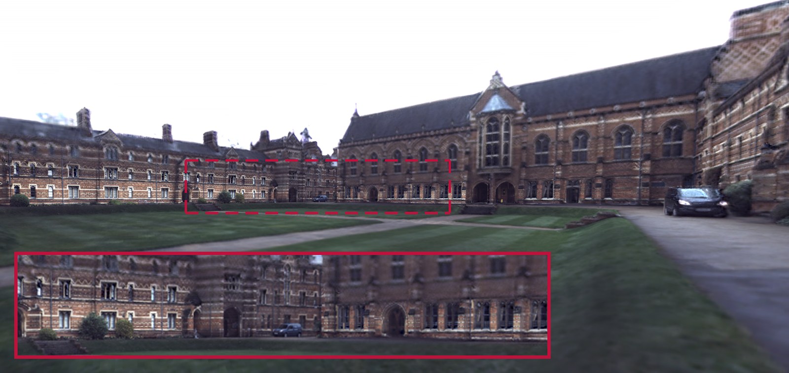
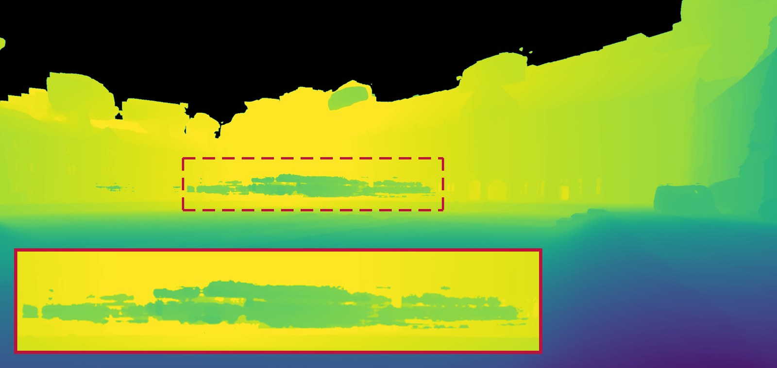
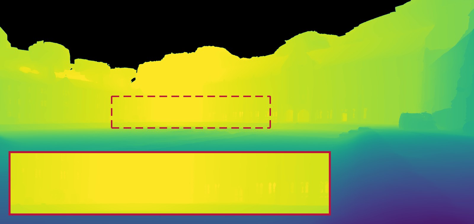
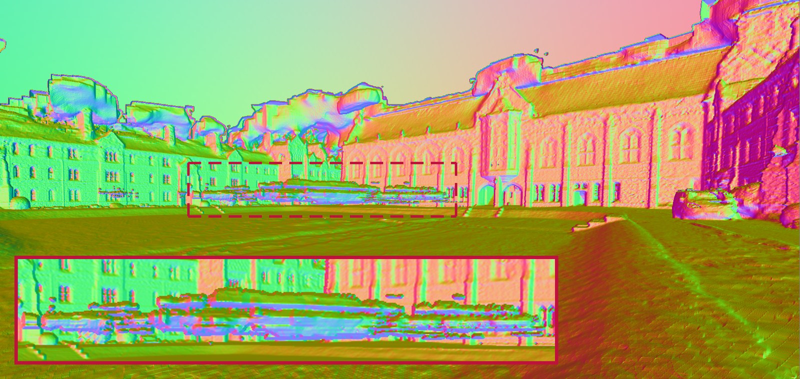
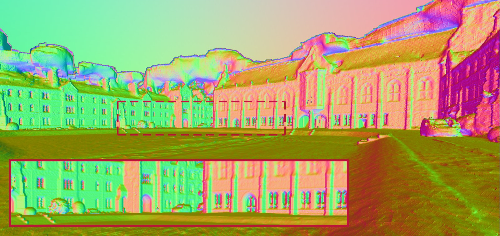
The same view on an Oxford Spires scene, from maps trained without and with occupied voxel guidance. The color images are nearly the same, but without the guidance the depth and normal maps show a band of floaters over the lawn.
3Map-driven camera optimization
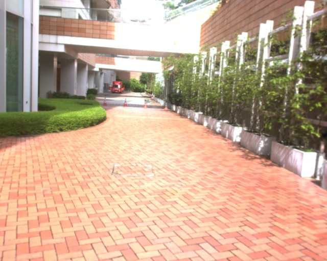
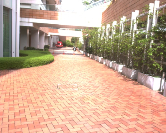
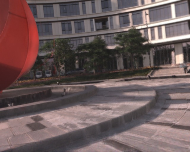
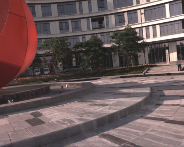
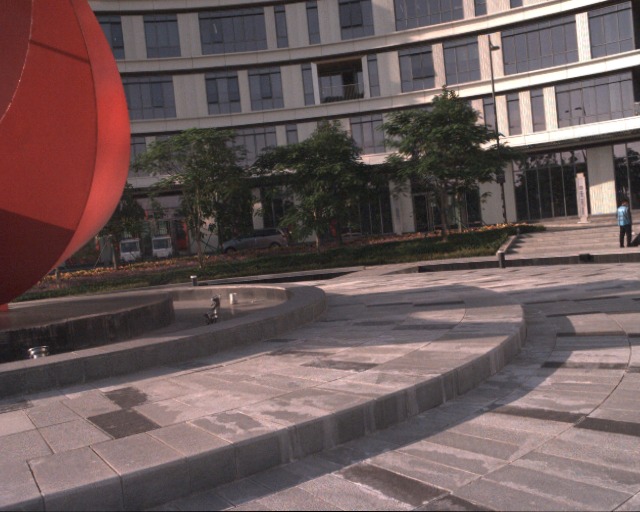
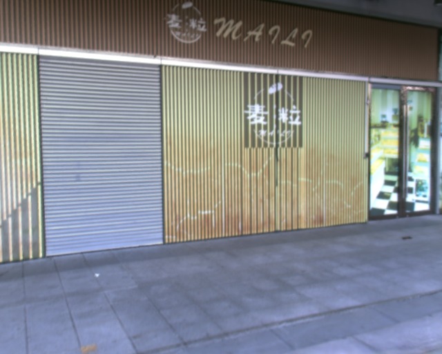
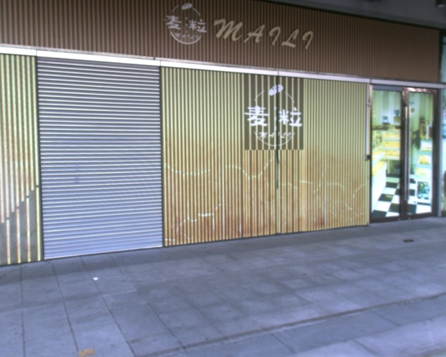
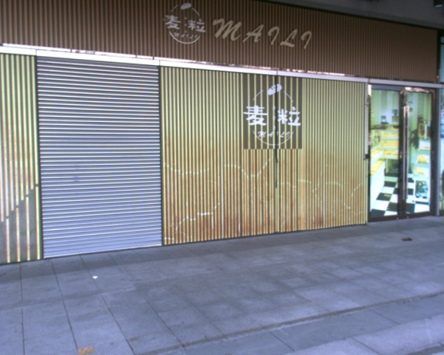
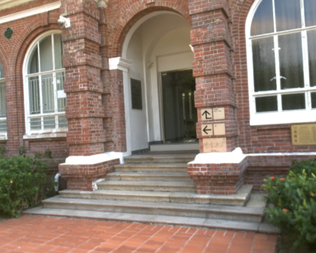
The cameras of robot data are metrically plausible but carry residual errors in every frame, and these errors blur the textures of the map. SpaRV alternates map training with photometric optimization of the pose and focal length of each camera against the current map. On the six FAST-LIVO2 scenes, camera optimization raises the training-view PSNR of SpaRV from 26.55 dB with the odometry cameras to 29.87 dB.
Show optimized cameras vs. ground truth
Show optimized cameras vs. ground truth
Show optimized cameras vs. ground truth

Show optimized cameras vs. ground truth
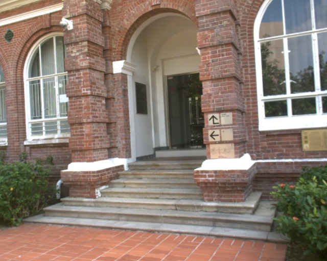
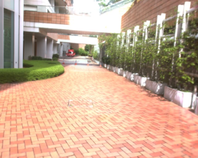
SpaRV on a FAST-LIVO2 training view, trained with the odometry cameras (left) and with the cameras it optimized (right).
| Method | Landmark | CBD | Culture | Drive | Sculpture | Street | Avg. |
|---|---|---|---|---|---|---|---|
| odometry cameras | |||||||
| InstantNGP | 31.705 | 25.312 | 23.131 | 18.379 | 25.276 | 23.429 | 24.539 |
| 3DGS | 32.260 | 22.033 | 21.571 | 25.570 | 24.294 | 26.836 | 25.427 |
| SVRaster | 31.616 | 26.419 | 24.749 | 26.035 | 24.636 | 26.025 | 26.580 |
| SpaRV | 31.223 | 25.923 | 24.681 | 26.871 | 24.483 | 26.130 | 26.552 |
| SpaRV (cam. opt.) | 36.190 | 28.114 | 26.512 | 29.817 | 28.548 | 30.007 | 29.865 |
| optimized cameras | |||||||
| InstantNGP | 31.693 | 25.182 | 24.064 | 19.622 | 25.290 | 23.596 | 24.908 |
| 3DGS | 36.256 | 23.159 | 21.231 | 27.006 | 27.937 | 30.657 | 27.708 |
| SVRaster | 36.011 | 28.680 | 24.755 | 27.587 | 28.411 | 29.443 | 29.148 |
| LetsGo | 32.066 | 27.107 | 24.218 | 17.712 | 23.177 | 28.408 | 25.448 |
| GS-SDF | 35.744 | 28.584 | 27.143 | 28.298 | 28.066 | 30.493 | 29.721 |
| SpaRV | 36.403 | 28.157 | 26.601 | 29.914 | 28.605 | 30.013 | 29.949 |
Odometry cameras: every method is trained on the FAST-LIVO2 odometry poses, and SpaRV (cam. opt.) also runs camera optimization. Optimized cameras: every method is trained on the cameras that SpaRV (cam. opt.) optimized.
4Large-scale reconstruction under bounded GPU memory
The GPU memory of a map grows with the extent of the scene. A single view, however, needs fine detail only near the camera, since distant regions project to few pixels. The octree of SpaRV keeps every coarser level that training passes through, and a coarser voxel needs no further optimization to be rendered as a level of detail. A granularity-driven cut selects voxels by the number of pixels they span on the image plane. It holds the submap in focus at the finest available level and the rest of the scene at coarser levels. The same cut rule serves training and rendering.

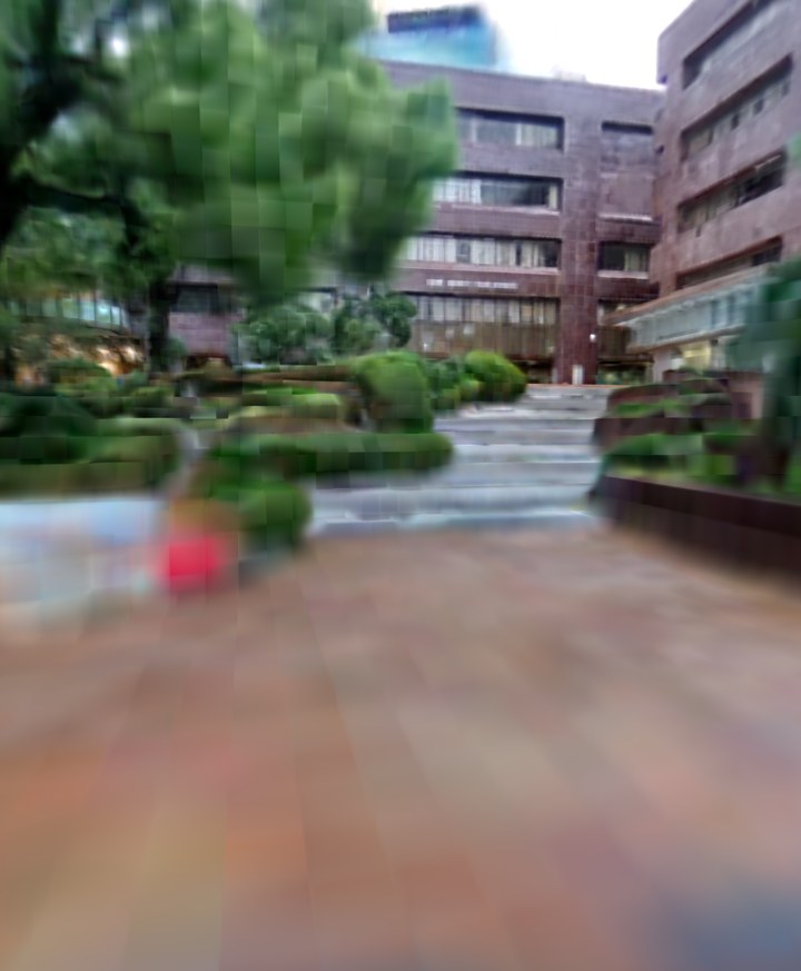
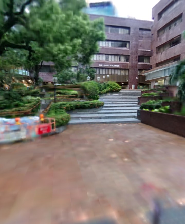
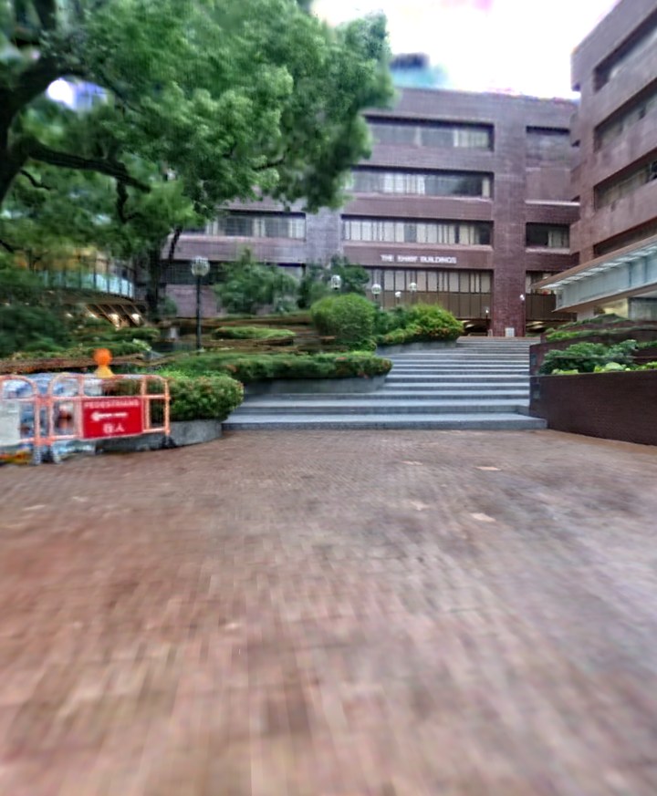
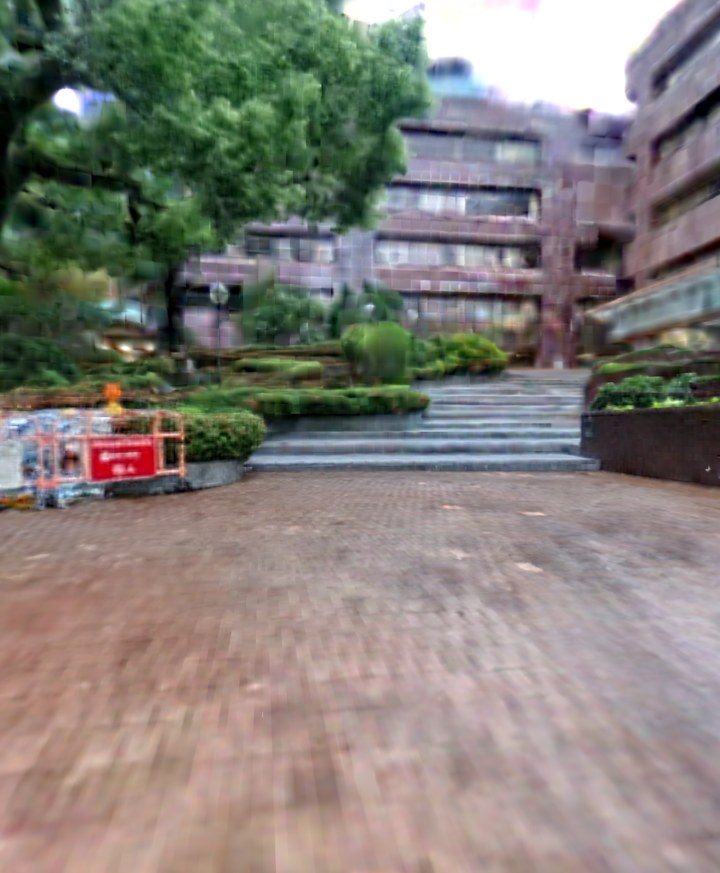
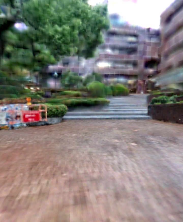
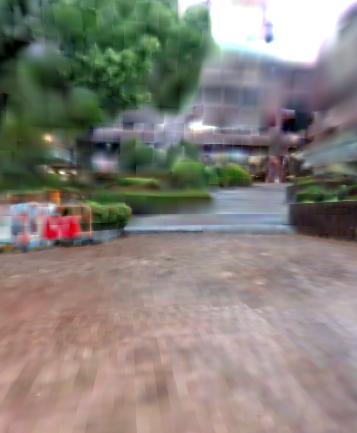
Levels of detail of one octree, seen from a single viewpoint. Top: increasingly fine levels. Bottom: cuts at an increasing granularity target τ, in pixels.
Results
We compare SpaRV with InstantNGP, 3DGS, SVRaster, LetsGo, and GS-SDF on synthetic indoor scenes and two outdoor LiDAR-visual datasets, with H3DGS on two large scenes we collected, and with EgoNeRF and OmniGS on an omnidirectional benchmark. In the tables, bold is the best result and underlined the second best.
Rendering away from the captured trajectory
A robot plans, simulates, and navigates beyond the views it captured, so the map is expected to stay geometrically consistent at those viewpoints. On FAST-LIVO2 Street, the methods are hard to tell apart at an interpolated view and separate once the camera moves off the captured trajectory. The image-only methods (InstantNGP, 3DGS, SVRaster) degrade. The Gaussian-based LetsGo and GS-SDF show popping on the billboard, where SpaRV stays consistent.
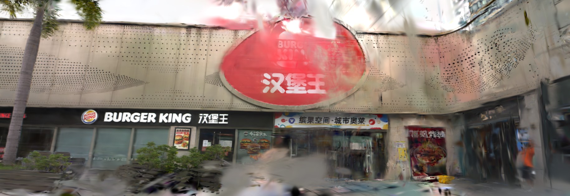
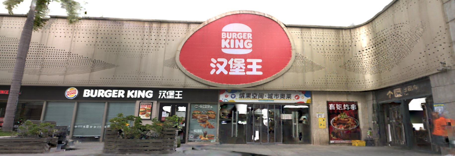
FAST-LIVO2 Street at an extrapolated view away from the captured trajectory. Pick a baseline and drag the divider.
Replica
Replica is a synthetic indoor dataset with ground-truth camera poses, which remove camera error from the comparison. We evaluate 8 scenes at interpolated viewpoints along the trajectory and at extrapolated viewpoints sampled uniformly in each scene. Pixels that no training view sees are excluded from the extrapolated evaluation.
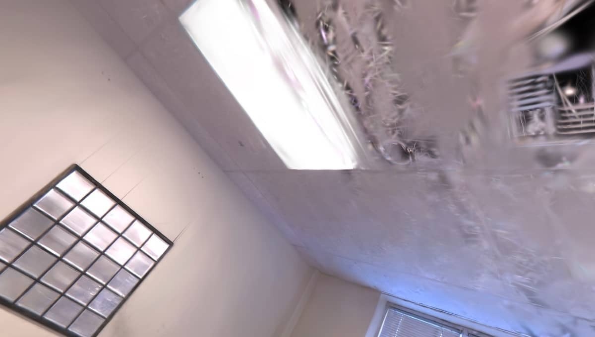
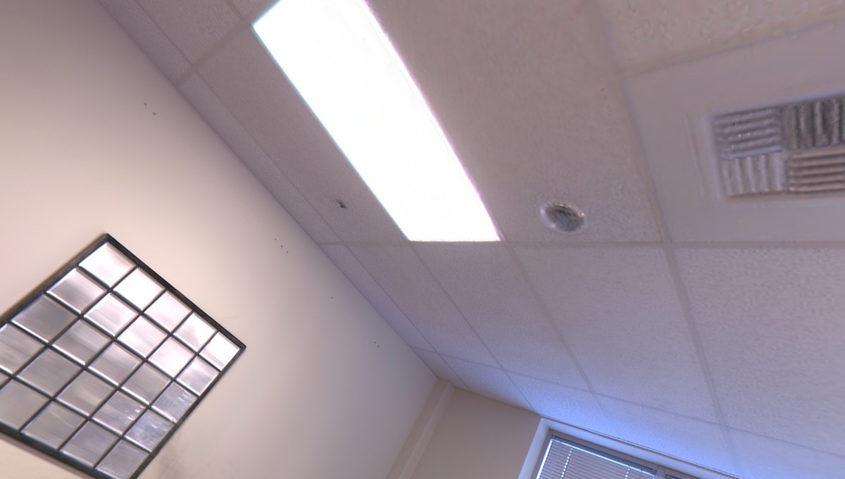
Replica Room-0. Every method is close to the reference at the interpolated training view; at the extrapolated view of the same maps, the methods separate.
| Method | Extrapolated (E) | Interpolated (I) | ||||
|---|---|---|---|---|---|---|
| PSNR↑ | SSIM↑ | LPIPS↓ | PSNR↑ | SSIM↑ | LPIPS↓ | |
| InstantNGP | 35.643 | 0.944 | 0.150 | 33.713 | 0.933 | 0.154 |
| 3DGS | 28.714 | 0.922 | 0.161 | 40.439 | 0.974 | 0.095 |
| SVRaster | 33.347 | 0.946 | 0.135 | 39.600 | 0.975 | 0.090 |
| LetsGo | 25.051 | 0.886 | 0.198 | 38.892 | 0.965 | 0.122 |
| GS-SDF | 36.053 | 0.962 | 0.103 | 40.548 | 0.973 | 0.078 |
| SpaRV | 36.690 | 0.963 | 0.077 | 41.001 | 0.982 | 0.047 |
FAST-LIVO2
FAST-LIVO2 is a real-world LiDAR-visual dataset captured with a solid-state Livox AVIA LiDAR. Its non-repetitive scan pattern makes the range measurements of each frame sparse and irregular. We use six outdoor scenes with three trajectory types: forward-facing (Landmark, CBD, Street), object-centric (Sculpture), and free-view (Culture, Drive). The initial cameras come from the FAST-LIVO2 odometry.
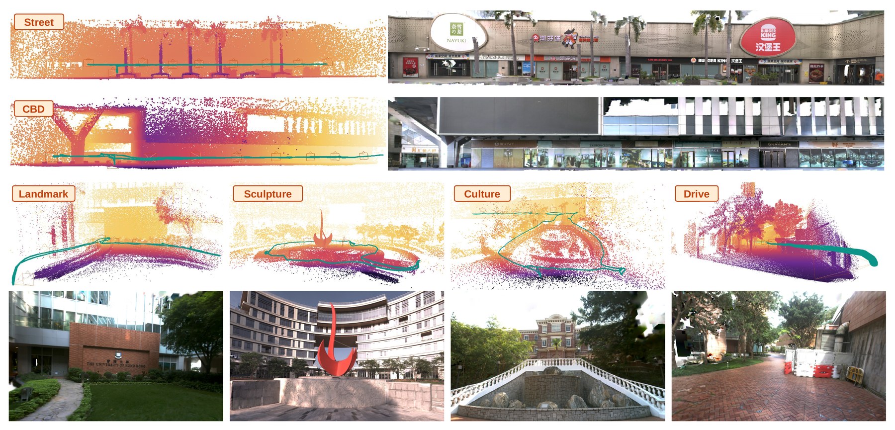
Fly-throughs along the test-view trajectory, with every method trained on the optimized cameras. Pick a scene and a baseline, and drag the divider.
On a test split that holds out one image in every eight, SpaRV has the lowest LPIPS on all six scenes and the highest SSIM on five of them. Its average PSNR is 0.13 dB below GS-SDF.
| Method | PSNR↑ | SSIM↑ | LPIPS↓ |
|---|---|---|---|
| InstantNGP | 25.350 | 0.761 | 0.325 |
| 3DGS | 27.198 | 0.845 | 0.224 |
| SVRaster | 28.042 | 0.873 | 0.168 |
| LetsGo | 28.395 | 0.881 | 0.164 |
| GS-SDF | 28.802 | 0.892 | 0.149 |
| SpaRV | 28.676 | 0.911 | 0.103 |
Oxford Spires
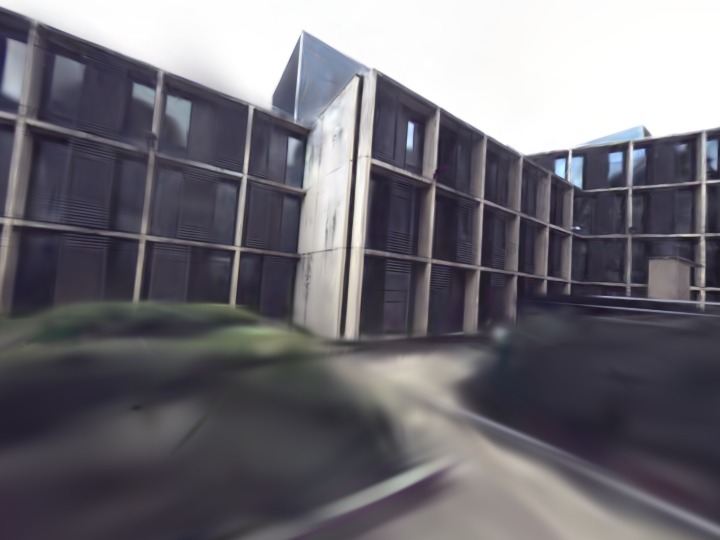
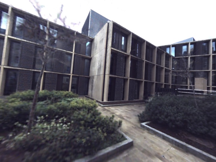
Oxford Spires has 12 outdoor sequences around Oxford landmarks, captured with a 64-channel Hesai QT64 LiDAR and three synchronized global-shutter cameras. Its ground-truth trajectories are registered against a millimeter-accurate laser scan, so this benchmark compares the methods with accurate cameras. SpaRV leads on all three averaged metrics, and its LPIPS is the lowest on all 12 sequences.
| Method | PSNR↑ | SSIM↑ | LPIPS↓ |
|---|---|---|---|
| InstantNGP | 24.102 | 0.772 | 0.428 |
| 3DGS | 25.759 | 0.796 | 0.366 |
| SVRaster | 25.286 | 0.814 | 0.302 |
| LetsGo | 25.714 | 0.835 | 0.304 |
| GS-SDF | 25.880 | 0.817 | 0.329 |
| SpaRV | 26.837 | 0.857 | 0.232 |
Large scenes: Garden and Campus
We captured Garden and Campus with a handheld scanner that carries a solid-state Livox MID360 LiDAR and three fisheye cameras. Garden is an outdoor district densely covered with complex objects: 44,550 images and 146.7 M LiDAR points along a 2,239 m trajectory. Campus spans an entire university: 63,582 images and 151.6 M LiDAR points along a 3,534 m trajectory. We compare SpaRV at two stages with H3DGS. SpaRV (coarse) is the output of coarse training, and SpaRV (deploy) adds submap training and renders through a cut around the camera.
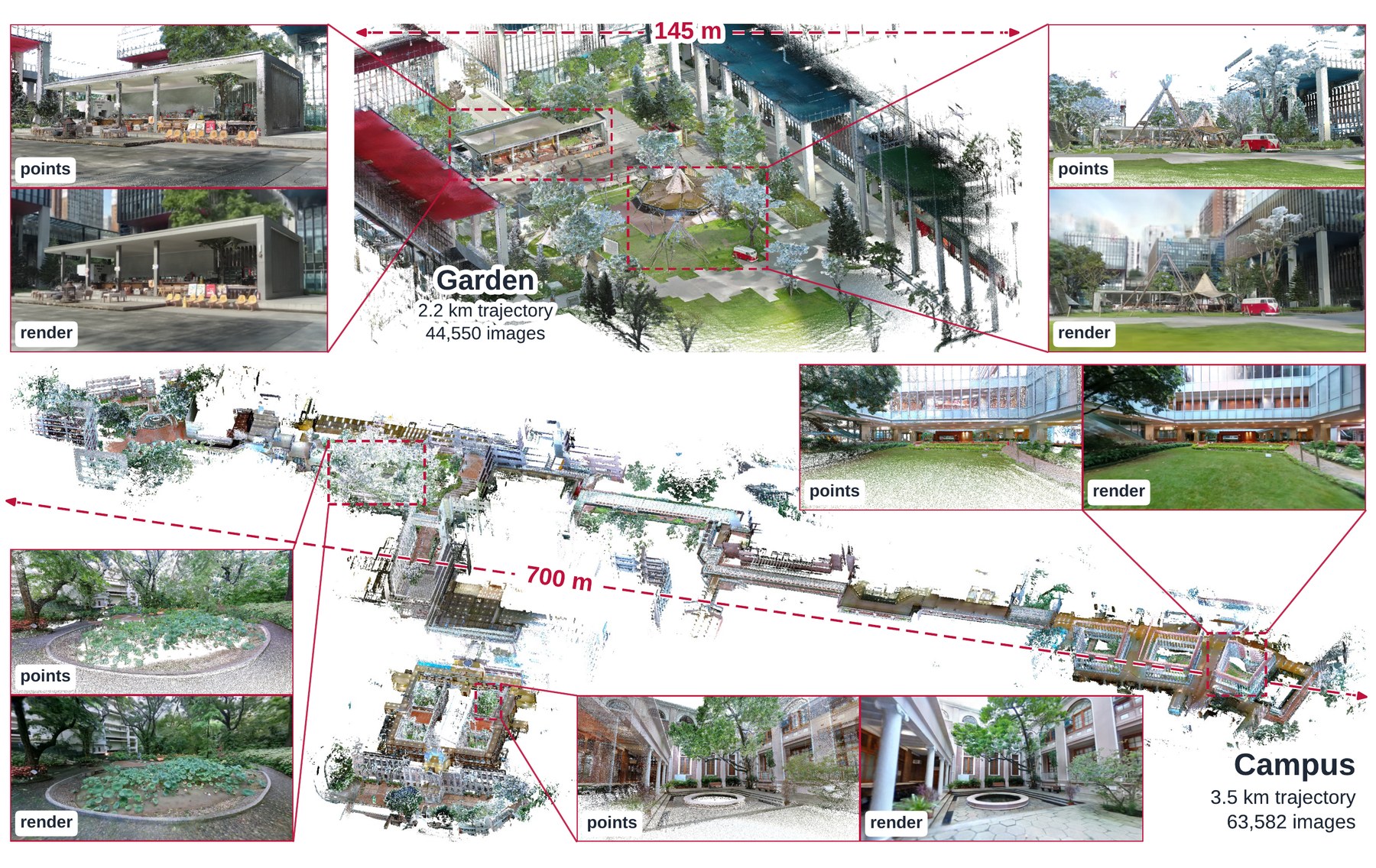
SpaRV (coarse), H3DGS, and SpaRV (deploy) along the whole fly-through of each scene. Campus plays at 2–3× speed.
Submap training improves SpaRV (coarse) on every metric, most on Campus (+2.5 dB PSNR). On Campus, SpaRV (deploy) renders at 68.8 FPS with a peak of 15.6 GiB of GPU memory, against 29.6 FPS and 22.5 GiB for H3DGS.
| Scene | Method | PSNR↑ | SSIM↑ | LPIPS↓ |
|---|---|---|---|---|
| Garden | H3DGS | 18.02 | 0.620 | 0.282 |
| SpaRV (coarse) | 20.89 | 0.712 | 0.346 | |
| SpaRV (deploy) | 21.12 | 0.713 | 0.295 | |
| Campus | H3DGS | 20.01 | 0.660 | 0.295 |
| SpaRV (coarse) | 20.62 | 0.652 | 0.451 | |
| SpaRV (deploy) | 23.16 | 0.760 | 0.283 |
| Method | Train [h]↓ | FPS↑ | Peak VRAM [GiB]↓ | |
|---|---|---|---|---|
| Train | Render | |||
| H3DGS | 7.3 | 29.6 | 8.3 | 22.5 |
| SpaRV (coarse) | 0.8 | 248.4 | 12.5 | 4.3 |
| SpaRV (deploy) | 8.7 | 68.8 | 11.7 | 15.6 |
Omnidirectional cameras: EgoNeRF
SpaRV renders equirectangular cameras with the same ray marcher, and uses the renderer and training schedule of the pinhole experiments unchanged. OmniGS, in contrast, specializes its rasterizer for the equirectangular camera. SpaRV outperforms OmniGS on all three metrics on both splits. The PSNR margin is small (0.34 dB on OmniBlender, 0.15 dB on Ricoh360), while LPIPS drops by 26% and 11%.
| Method | OmniBlender (11 scenes) | Ricoh360 (11 scenes) | ||||
|---|---|---|---|---|---|---|
| PSNR↑ | SSIM↑ | LPIPS↓ | PSNR↑ | SSIM↑ | LPIPS↓ | |
| EgoNeRF | 30.93 | 0.892 | 0.207 | 24.89 | 0.752 | 0.353 |
| OmniGS | 33.09 | 0.918 | 0.174 | 25.99 | 0.825 | 0.262 |
| SpaRV | 33.43 | 0.926 | 0.129 | 26.14 | 0.838 | 0.233 |
Applications
Sensor simulation
The ray marcher accepts arbitrary rays, so one trained map can render other cameras and LiDARs. From the Garden map, SpaRV renders three camera models (pinhole, fisheye, and omnidirectional) and three LiDAR scan patterns (Livox AVIA, Livox MID360, and an OS128-style ring pattern).
Mesh extraction


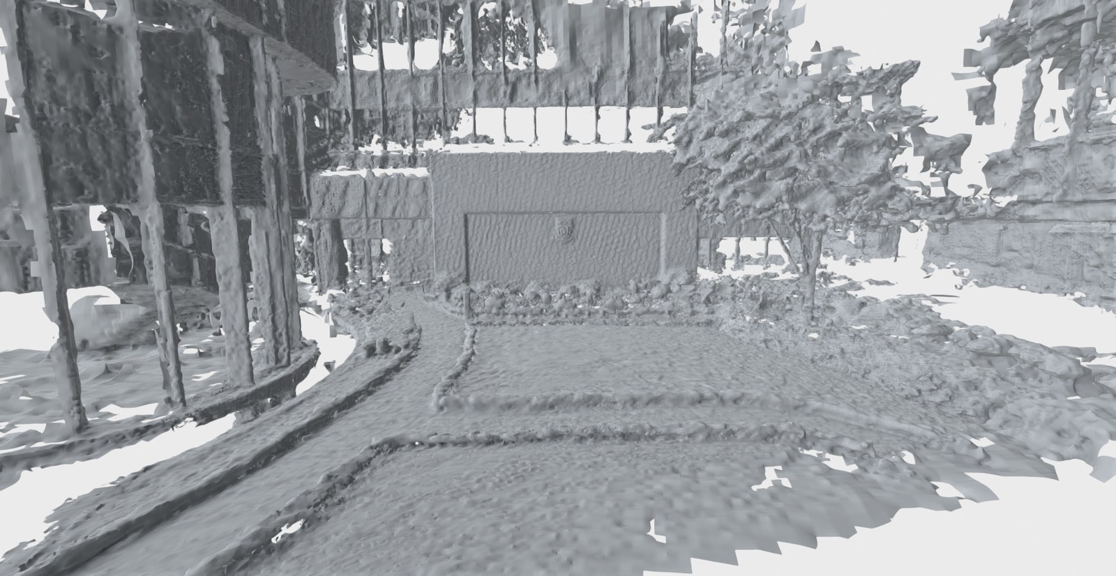
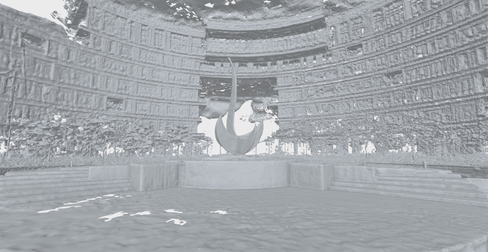
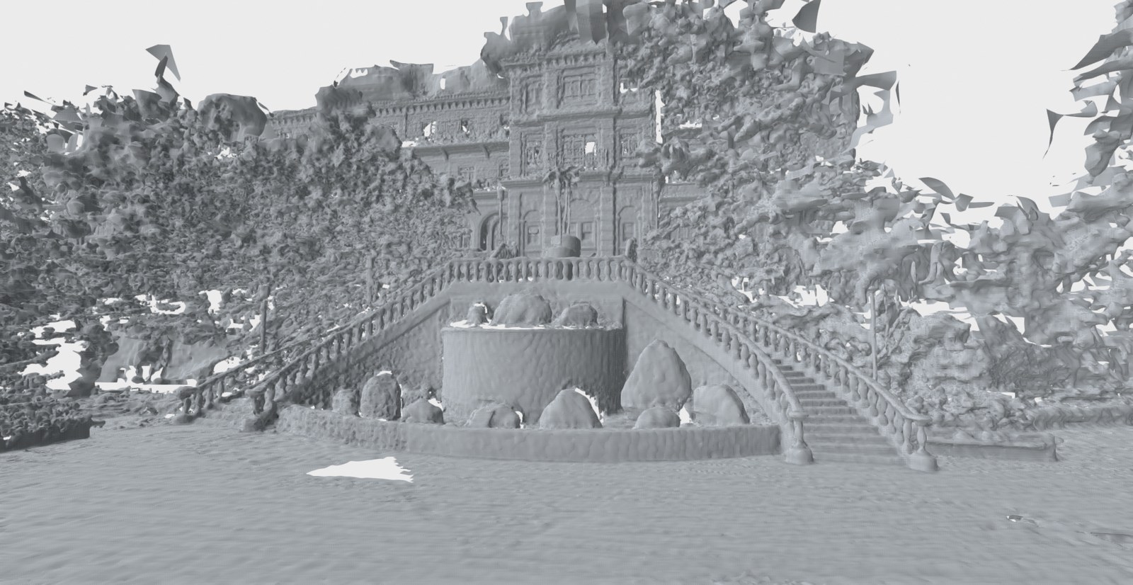
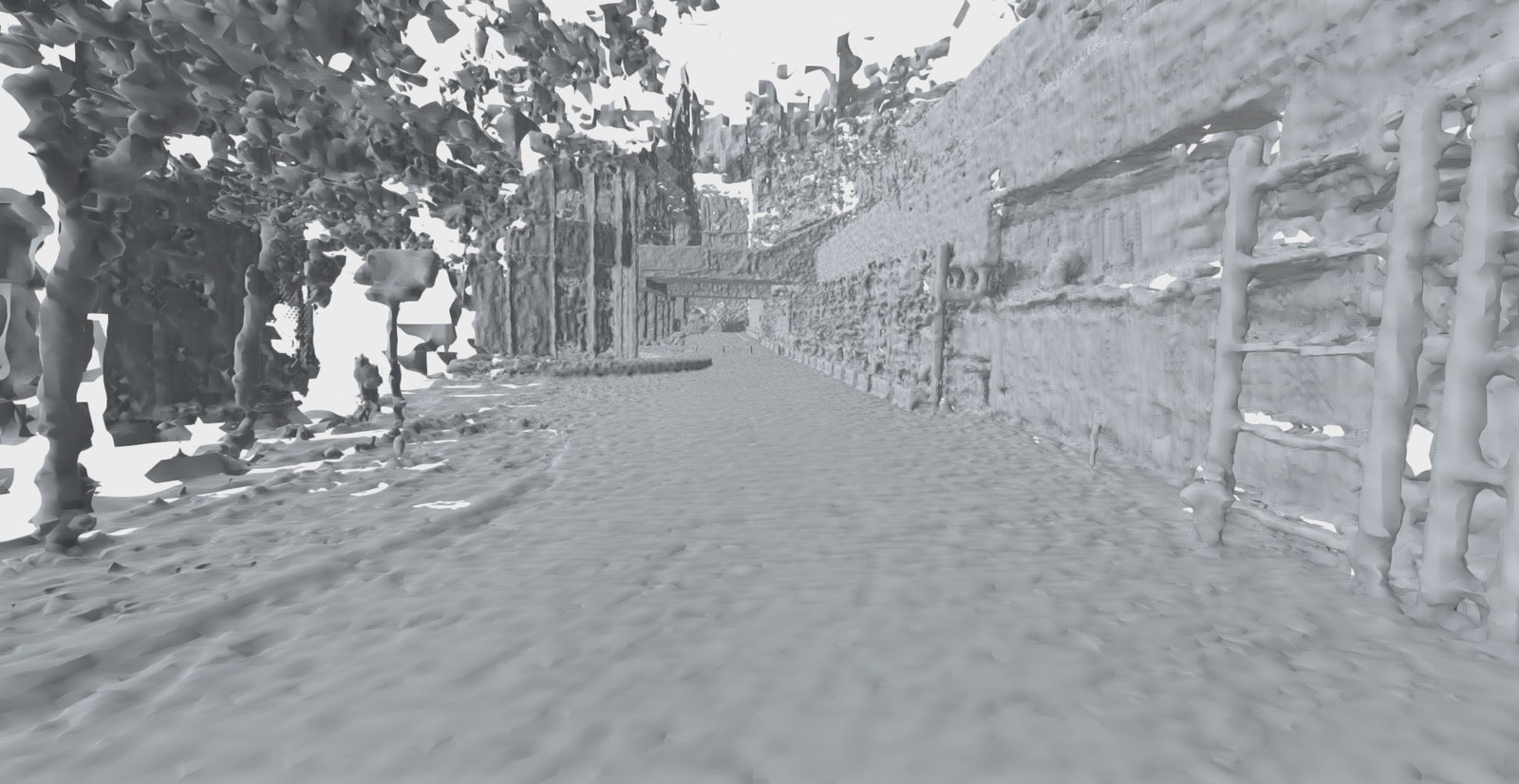
Meshes extracted from the six FAST-LIVO2 maps by marching cubes.
BibTeX
@misc{liu2026sparv,
  title   = {SpaRV: Sparse Radiance Voxels for Scalable Geometrically Consistent LiDAR-Visual Mapping and Rendering},
  author  = {Liu, Jianheng and Wan, Yunfei and Cheng, Fangming and Hong, Xiangyu and Zou, Zuhao and
             Li, Haotian and Yin, Longji and Zheng, Chunran and Lin, Jiarong and Zhang, Fu},
  note    = {Under review},
  year    = {2026}
}